To calculate the phon (vibrational) properties we will use the phonon code of the Quantum Espresso package.
The single atoms don't have phonon properties and only molecules and crystals have. We will take the example of methane molecule and Diamond crystal.
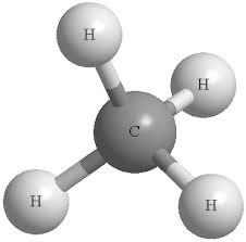
Example 01: Methane CH4 ( Vibrational Modes of Methane )
We’ll start by calculating the vibrational modes of a molecule. This calculation is set up in 2 parts:
A self consistent calculation of the density and wavefunction. You might notice this is often the first step in many of the calculations we do.
A DFPT calculation of the dynamical matrix and normal modes. As we have a molecule, we only need look at the gamma point here.
There are three things you should take note of though:
We’ve specified the gamma point only by asking for a 1x1x1 unshifted grid, whereas previously we’ve usually explicitly asked for the gamma point. This latter option uses optimizations that can make the calculation a bit faster if we only use the gamma point, however it does not generate output that is compatible with the subsequent DFPT calculation of the frequencies, so we instead specify the gamma point in the manner done in the file.
We’ve re-oriented the molecule relative to what you’ve seen previously, and the atomic positions have also been optimized. By specifying the atoms in this manner, where the components of the hydrogens along each direction have the same magnitude but different signs, the code is much better able to detect the symmetry of the molecule. This is very important for calculations of the vibrations. If the code understands that all the hydrogen atoms are equivalent by symmetry, it need only calculate the derivatives of the energy with respect to one of the hydrogen positions, and then it can populate the full dynamical matrix based on the symmetry of the system.
We’ve increased the default value of ecutrho which is usually four times the value of ecutwfc. This can help alleviate some issues with acoustic mode frequencies at gamma mentioned below.
Input files
We need 4 files
algerien1970@linux-wipm:~/abinitio/QE-tutorials/CH4_Phon> ls
CH4.ph.in  CH4.scf.in  C.pbe-rrkjus.UPF  H.pbe-rrkjus.UPF
CH4.scf.in
 &CONTROL
    pseudo_dir = './'
 /

 &SYSTEM
    ibrav = 1
    A = 10.0
    nat = 5
    ntyp = 2
    ecutwfc = 25.0
    ecutrho = 200.0
 /

 &ELECTRONS
 /

ATOMIC_SPECIES
 C  12.011  C.pbe-rrkjus.UPF
 H   1.008  H.pbe-rrkjus.UPF

ATOMIC_POSITIONS angstrom
 C  0.0           0.0           0.0
 H  0.634532333   0.634532333   0.634532333
 H -0.634532333  -0.634532333   0.634532333
 H  0.634532333  -0.634532333  -0.634532333
 H -0.634532333   0.634532333  -0.634532333

K_POINTS automatic
1 1 1  0 0 0
CH4.ph.in
phonons of CH4 (gamma only)
 &INPUTPH
  tr2_ph = 1.0d-15
  asr = .true.
 /
0.0 0.0 0.0
C.pbe-rrkjus.UPF and C.pbe-rrkjus.UPF
You can download the files using the following command
$ wget https://www.quantum-espresso.org/upf_files/C.pbe-rrkjus.UPF --no-check-certificate
$ wget https://www.quantum-espresso.org/upf_files/O.pbe-rrkjus.UPF --no-check-certificate
SCF calculation
algerien1970@linux-wipm:~/abinitio/QE-tutorials/CH4_Phon> pw.x < CH4.scf.in |tee CH4.scf.out
Phonon calculation
algerien1970@linux-wipm:~/abinitio/QE-tutorials/CH4_Phon> ph.x < CH4.ph.in |tee CH4.ph.out
Output files
File matdyn (the name of this file can be changed in the input file)
This
file stores the dynamical matrix, which can then be passed to several
other codes for further analysis. Take a look at it now.
The
top of the file has the atoms, their masses (in internal units) and
positions. This is followed by the dynamical matrix (3x3 complex numbers
for each possible pair of atoms - all the imaginary parts are zero at
gamma).
Finally the frequencies of each calculated vibrational
mode, both in THz and cm-1 are given along with the corresponding
wavevector. A molecule with 5 atoms will have 15 possible vibrational
modes.
Directory _ph0
contains intermediate and restart data for the ph.x calculation.
Now let’s look through the output of the ph.x calculation.
Near the top you’ll see an analysis of the number of calculations that need to be done given the symmetry of the system. You’ll note that only 3 of the 15 total representations need to be explicitly calculated. This is why it’s so important to have the code detect the symmetry of your system correctly. Potentially the calculation could have been 5 times slower.
This is followed by a self consistent calculation for each of the representations that need to be calculated.
Then we have the frequencies obtained by diagonalizing the dynamical matrix.
Finally we have a symmetry analysis of the resulting modes, giving the mode symmetry and whether they should be detectable by Raman or infrared spectroscropy or both.
You’ll likely have noticed we have 3 quite negative frequencies. These are the rotational modes of the molecule. It’s difficult to get these to come out to be zero in the DPFT calculation. In principle this could be enforced by a suitable constraint in the code, but this is not available in ph.x. It’s possible in some other codes however.
The subsequent three modes near zero are the three translational modes, and these have been enforced to be close to zero by the asr setting in the input file.
Note as the frequency is calculated using the square root of the curvature of the energy, a negative frequency is in fact a convention used to indicate that the frequency is imaginary, and the energy curvature is negative. This can indicate some instability in the system, so it is good to ensure you are starting from an optimized structure as you learned how to do last week.
Example 02: Carbon Diamond (Phonon Bandstructure and DOS of Carbon Diamond)

Now that you’ve seen how to calculate the frequencies at a single wavevector, the next step is to calculate the phonon band dispersion of a crystal.
This calculation has five steps:
- Perform self-consistent calculation of the density and wavefunction.
- Calculate the dynamical matrix on a set of wavevectors. I’ll call these q-points from here on, and use k-points to refer to electronic wavevectors.
- Fourier transform our grid of dynamical matrices to obtain a set of real space force constants.
- Perform an inverse Fourier transform of the real space force constants to obtain the dynamical matrix at an arbitrary q-point. This allows us calculate mode frequencies for a fairly dense set of points along lines between high-symmetry points in the same manner as for the electronic band structure.
- Generate the plot.
First examine the scf input file Diamond.scf.in. This is similar to those
we’ve seen before. This time we’ve specified prefix. This can be useful if
you’ve got different calculations in the same directory. Again, we’ve
increased ecutrho from its default. The rest is as before.
Now examine the ph.x input file Diamond.ph.in
- This is structured as before, but now:
- We have specified the same prefix as in the scf input file
- We’ve set
ldisp = .true.which says we’re going to calculate a grid of q-points. nq1,nq2andnq3define our q-point grid then.
- This is structured as before, but now:
Input files
We need 6 files
algerien1970@linux-wipm:~/abinitio/QE-tutorials/Diamond_phon> ls
C.pbe-rrkjus.UPF  Diamond.matdyn-dos.in  Diamond.matdyn-bands.in  Diamond.ph.in  Diamond.scf.in
Diamond.q2r.in
Diamond.scf.in
 &CONTROL
    pseudo_dir = './'
    prefix = 'Diamond'
    disk_io = 'low'
 /

 &SYSTEM
    ibrav =  2
    A = 3.567
    nat = 2
    ntyp = 1
    ecutwfc = 60.0
    ecutrho = 400.0
 /

 &ELECTRONS
 /

ATOMIC_SPECIES
 C  12.011  C.pbe-rrkjus.UPF

ATOMIC_POSITIONS crystal
 C 0.00 0.00 0.00
 C 0.25 0.25 0.25

K_POINTS automatic
  8 8 8 0 0 0
Diamond.ph.in
phonons of Carbon diamond on a grid
 &INPUTPH
  prefix = 'Diamond',
  asr = .true.
  ldisp = .true.
  nq1=4, nq2=4, nq3=4
 /
Diamond.q2r.in
    &input
fildyn = 'matdyn'
zasr = 'simple'
flfrc = 'Diamond444.fc'
/
Diamond.matdyn-bands.in
    &input
asr = 'simple'
flfrc = 'Diamond444.fc'
flfrq = 'Diamond-bands.freq'
dos=.false.
q_in_band_form=.true.
/
8
0.000 0.000 0.000 30
0.375 0.375 0.750 10
0.500 0.500 1.000 30
1.000 1.000 1.000 30
0.500 0.500 0.500 30
0.000 0.500 0.500 30
0.250 0.500 0.750 30
0.500 0.500 0.500 0
Diamond.matdyn-dos.in
    &input
    asr='simple'
    flfrc='Diamond444.fc'
    flfrq='Diamond-dos.freq'
    dos=.true.,
    nk1=20,nk2=20,nk3=20
    fldos='Diamond-q20.dos'
 /
C.pbe-rrkjus.UPF
You can download the file using the following command
$ wget https://www.quantum-espresso.org/upf_files/C.pbe-rrkjus.UPF --no-check-certificate
SCF calculation
algerien1970@linux-wipm:~/abinitio/QE-tutorials/CH4_Phon> pw.x < Diamond.scf.in |tee Diamond.scf.out
Phonon calculation
algerien1970@linux-wipm:~/abinitio/QE-tutorials/CH4_Phon> ph.x < Diamond.ph.in |tee Diamond.ph.out
Once complete you’ll see several files have been generated in the calculation directory.
matdyn0has the q-point grid used followed by a list of the q-points at which the dynamical matrix has been calculated.matdyn1,matdyn2, etc is the dynamical matrix at each calculated q-point as before.
Now take a look through the main output file.
- You’ll see it’s quite similar to the methane case, but now contains a section for each calculated q-point where it figured how how many represenations need to be calculated based on the symmetry, an scf cycle for each, and the frequencies and mode symmetries obtained by diagonalizing the dynamical matrix at that q-point.
- It’s good to look through this file and ensure you’re getting reasonable numbers for the frequencies before proceeding.
Calculation of real space force constants
Next we’ll be generating the real space force constants from our grid of dynamical matrices using the q2r.x code.
algerien1970@linux-wipm:~/abinitio/QE-tutorials/Diamond_phon> q2r.x < Diamond.q2r.in |tee Diamond.q2r.out
The output isn’t particularly interesting. The Diamond444.fc file has the
force constants for each pair of atoms in each direction for each of the
4x4x4 unit cells in real space.
Calculation of Phonon Band Structure
Finally we want to use this to generate our normal mode dispersion. We’ll be
doing this with the matdyn.x code. As with q2r.x this doesn’t have a doc
file describing its input variables. But you can check the comments at the
top of its source file to get their details. On the mt-student server this
is at /opt/build/quantum-espresso/q-e-qe-6.3/PHonon/PH/matdyn.f90.
Take a look at our input file Diamond.matdyn-bands.in.
Here we’re setting:
asrto again tell it to try to force the acoustic modes at gamma to go to zero.flfrcto give it the name of the file with the real space force constants from theq2r.xcalculation.flfrqto give it the name of the output file to store its calculated frequencies.dosto tell it we’re not calculating a density of statesq_in_band_formto tell it we want to calculate bands between high symmetry points.- We finally give it a number and list of high symmetry points with the number of points to calculate along each line, in the same way as we did for the electronic band structure.
algerien1970@linux-wipm:~/abinitio/QE-tutorials/Diamond_phon> matdyn.x < Diamond.matdyn-bands.in |tee Diamond.matdyn-bands.out
There’s very little actual output from the code itself, but it will generate the files
Diamond-bands.freqandDiamond-bands.freq.gp. Both of which contain the frequencies along the lines we requested. Now we need to turn it into a plot.Finally we want to generate a plot of these frequencies. We could do that directly with the previous output:
Diamond-bands.freq.gpis a multicolumn space separated list of the frequencies in cm-1.- It can be easier to use the
plotband.xtool to help generate a plot. - Call this with
plotband.x Diamond-bands.freq. This will then ask you for an Emin and Emax value - you should pick values equal to or below and above the numbers it suggests. Then it will ask you for an output file name. Pick “Diamond-bands-gpl.dat” here. You can then cancel further running of this code withctrl+c. Note it has output the location of the high-symmetry points along its x-axis.
- It can be easier to use the
Once you’ve done this, a gnuplot script
plotbands.gplthas been provided that you can use to generate the band structure plot. This is very similar to the one used for the electronic band structure, but the location of the high-symmetry points along the x-axis has changed as has the name of the data file we’re plotting. Run this withgnuplot plotbands.gplt.
algerien197@linux-wipm:~/abinitio/QE-tutorials/Diamond_phon> plotband.x
     Input file > Diamond-bands.freq
Reading    6 bands at    191 k-points
Range:    0.0000 1302.5970eV  Emin, Emax, [firstk, lastk] > 0.0000 1302.5970
high-symmetry point:  0.0000 0.0000 0.0000   x coordinate   0.0000
high-symmetry point:  0.5000 0.5000 1.0000   x coordinate   1.2247
high-symmetry point:  1.0000 1.0000 1.0000   x coordinate   1.9319
high-symmetry point:  0.5000 0.5000 0.5000   x coordinate   2.7979
high-symmetry point:  0.0000 0.5000 0.5000   x coordinate   3.2979
high-symmetry point:  0.2500 0.5000 0.7500   x coordinate   3.6514
high-symmetry point:  0.5000 0.5000 0.5000   x coordinate   4.0050
output file (gnuplot/xmgr) > Diamond-bands-gpl.dat
bands in gnuplot/xmgr format written to file Diamond-bands-gpl.dat
output file (ps) >
stopping ...
Plotting Band Structure
gnuplot> plot "Diamond-bands-gpldat.dat" using 1:2 with lines

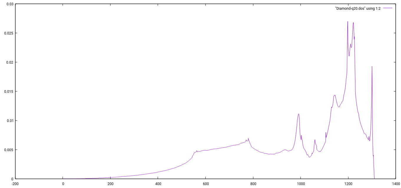
Calculation of Phonon DOS
algerien1970@linux-wipm:~/abinitio/QE-tutorials/Diamond_phon> matdyn.x < Diamond.matdyn-dos.in |tee Diamond.matdyn-dos.out
Plotting VDOS
gnuplot> plot "Diamond-q20.dos" using 1:2 with lines
Reference: https://eamonnmurray.gitlab.io/modelling_materials/lab06/
For comparaison check the following links:
http://openmopac.net/manual/diamond/Diamond%20Phonon%20Walk%20from%20BZ.html
http://exciting.wikidot.com/oxygen-phonon-properties-diamond
https://www.scm.com/doc/Tutorials/StructureAndReactivity/DiamondOptimizationAndPhonons.html
https://www.esrf.fr/UsersAndScience/Publications/Highlights/2001/CAD/CAD2.html


![[QE-users] Script to produce explicit q points along BZ paths for input in matdyn.x](https://lh3.googleusercontent.com/blogger_img_proxy/AEn0k_tlLrg0B2y_g_gz4O5-Ca_9Vp27_yWzLqsDPgIRCQpuDmTJirDINtv_ETx6OnWHk1pdnqhCQwLmr4InD45n9R6xUe7xtnzsJ3IULFPT4KvGFwb78znO-Vzm59BuUDjHWPFiN1nvU8BwK47vw7jLE3Za1MgGhYCoMfHCemNSXLgMSC2BqIHI5iv4V0OP18v83ub5v6FrxId7hw=w100)

0 Comments