Draw GaAs band structure using Quantum ESPRESSO

MateriApps Development Team

Introduction

Quantum ESPRESSO is open-source software for first-principles calculation. The detailed documentations and many related tools are open on the Web. In addition, because it uses a plane wave basis, there are few control parameters that determine the calculation accuracy. It is one of the best software for beginners to try first principles calculation.

In this review, we will calculate the band of a typical semiconductor GaAs, and briefly explain how to write a band diagram. We have used the environment of MateriApps Live! ver. 3.3. The version of the Quantum ESPRESSO is 6.7. In writing this article, I referred to the following tutorial.

http://www.cmpt.phys.tohoku.ac.jp/~koretsune/SATL_qe_tutorial/

How to run

The calculation will be faster if you increase the number of CPUs as much as possible in advance in the setting of VirtualBox. Before launching MateriApps LIVE!, you can change the number of CPU processors by going to “Settings<System<Processors”. (Check the number of CPU cores on your PC and keep it the same. Normally you should set it to the maximum within the green bar on the CPU number selection screen.) Next, launch the terminal on MateriApps LIVE! (From Start Menu, “System Tools” > “LXTerminal”).

Next, download and extract the script files that was prepared in advance for easy execution.

$ wget https://github.com/cmsi/malive-tutorial/releases/download/tutorial-20210520/qe_GaAs.tgz
$ tar zxvf qe_GaAs.tgz
$ cd qe_GaAs

To preform electronic state calculation, it is necessary to use an appropriate pseudopotential file for each atom. Pseudopotentials can be found and downloaded from this page. Here, for downloading, it is only necessary to type as follows:

$ wget https://www.quantum-espresso.org/upf_files/Ga.pbe-dn-kjpaw_psl.1.0.0.UPF
$ wget https://www.quantum-espresso.org/upf_files/As.pbe-n-kjpaw_psl.1.0.0.UPF

To perform band calculation, execute the following command from the terminal.

$ pw.x < GaAs.scf.in > GaAs.scf.out
$ pw.x < GaAs.nscf.in > GaAs.nscf.out
$ bands.x < GaAs.band.in > GaAs.band.out
$ gnuplot -persistent plot.gp

The calculation should take a few minutes. If multiple calculation cores can be used, type, for example,

mpirun -np 2 pw.x < GaAs.scf.in > GaAs.scf.out

Then, parallel calculations using two CPU cores will start, making the calculation earlier.

The meaning of each command is as follows:

Self-consistent calculation using pw.x
Non-self-consistent calculation using pw.x
Post-processing using bands.x
Drawing a band diagram using gnuplot

The calculation takes several minutes. When the calculation is completed successfully, the following band diagram should be displayed.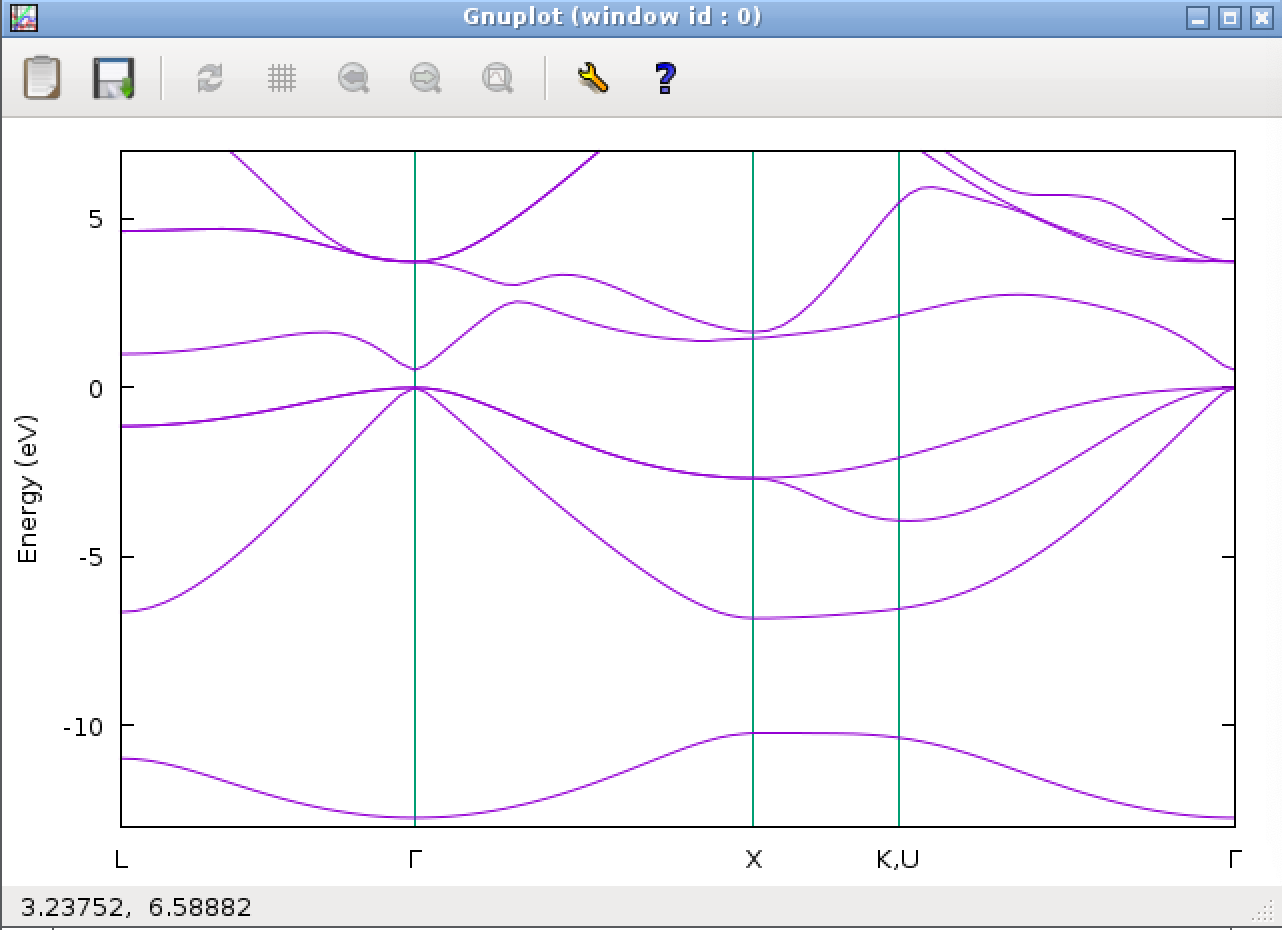

Explanation of the input file: Self-consistent calculation

Let’s take a closer look at the contents of the input file (GaAs.scf.in) for self-consistent calculation. Let’s look at the first part.

&control
calculation = 'scf'
prefix = 'GaAs'
pseudo_dir = './'
wf_collect = .true.
/

From &control to / are grouped together, and between them parameters are set in the format of “parameter name = value”. The “calculation” parameter specifies the calculation mode. Here it is ‘scf’. This means self-consistent calculation (solving the Kohn-Sham equation self-consistently). The “prefix” parameter specifies the header for output files. It is a good idea to specify a material name. Here, it is ‘GaAs’. The “pseudo_dir” parameter is the location of the pseudopotential file. Now the pseudopotential files are located in the same working directory, so for now we’ll use ‘./’ (meaning the present working directory). The “twf_collect” parameter is an option to save the wave function.

&system
ibrav = 2
celldm(1) = 10.6867
nat = 2
ntyp = 2
ecutwfc = 60
ecutrho = 244
/

This paragraph is a part that expresses the characteristics of the system. “ibrav” is a way to specify the Bravais lattice, and “ibrav = 2” specifies the unit cell vector of fcc. GaAs has the Zinc-Blende crystal structure, in which Ga and As are arranged in two sublattices of the diamond lattice. The unit lattice vector of the diamond lattice is the same as fcc. Let’s watch out. “celldm(1)” represents the lattice constant, “nat” represents the number of atoms in the unit cell, and “ntyp” represents the number of elements. “ecutwfc” and “ecutrho” are the cutoff energies (unit is Rydberg). Increasing the cutoff value, increases the accuracy, but makes the calculation heavier. The recommended value depends on the type of pseudopotential. Here we set the recommended value described at the beginning of the pseudopotential file.

&electrons
mixing_mode = 'plain'
mixing_beta = 0.7
conv_thr = 1.0d-8
diago_david_ndim = 4
/

This paragraph specifies the parameters for the convergence of the wave function. “conv_thr” is a parameter used for convergence judgment. “mixing_mode” and “mixing_beta” are parameters to speed up convergence, but for light calculations you do not have to worry too much. Please refer to official page for details.

ATOMIC_SPECIES
Ga 69.723 Ga.pbe-dn-kjpaw_psl.1.0.0.UPF
As 74.921595 As.pbe-n-kjpaw_psl.1.0.0.UPF

This part specifies the atom type and atomic weight (not used in the present calculation) and the pseudopotential file. Quantum ESPRESSO uses a method called the pseudopotential method, which does not deal with inner core electrons, but instead replaces the effect of inner shell electrons on valence electrons with the pseudopotential. This can greatly reduce the amount of calculation, but the result depends on the choice of pseudopotential. Therefore, the pseudopotential must be carefully selected. As already mentioned, pseudopotentials can be downloaded from the page in Quantum ESPRESSO .

ATOMIC_POSITIONS
Ga 0.00 0.00 0.00
As 0.25 0.25 0.25

This represents the internal coordinates (xyz coordinates) in the Ga and As unit cells.

K_POINTS {automatic}
8 8 8 0 0 0

The last part specifies the number of points (k points) in the wavenumber vector. The first three numbers specify the number of wavenumber divisions in the x, y, and z directions. If {automatic} is specified, k points are automatically taken discretely in the first Brillouin zone. The last three numbers describe the wave number origin shift. Here, there is no shift (all 0). The more k points the more accurate the calculation, but the slower the calculation. In the self-consistent calculation, it takes time to repeat the calculation until the electron density converges, so the number of k points is small.

Explanation of the input file: Non-self-consistent calculation

Self-consistent calculations can provide sufficiently accurate electron density, but there are not enough k points to write a band diagram. Therefore, based on the electron density obtained by self-consistent calculation, band calculation is performed for many k points on the line segment of the reciprocal lattice space to be obtained. The input file (GaAs.nscf.in) is almost the same as the file (GaAs.scf.in) used in the self-consistent calculation. Only the changes are described below. In the first part,

&control
calculation = 'bands'
prefix = 'GaAs'
pseudo_dir = './'
wf_collect = .true.
/

the parameter “calculation” is set to ‘bands’. As a result, the self-consistent calculation is not performed, and band calculation is performed in a non-self-consistent manner. In the system part,

&system
ibrav = 2
celldm(1) = 10.6867
nat = 2
ntyp = 2
ecutwfc = 60
ecutrho = 244
nbnd = 16
/

In the last line, the parameter “nbnd” is added (the number of the bands to be plotted). The last k-point designation has been changed to

K_POINTS {crystal_b}
5
 0.00  0.50  0.00  20 !L
 0.00  0.00  0.00  30 !G
-0.50  0.00 -0.50  10 !X
-0.375 0.00 -0.675 30 !K,U
 0.00  0.00 -1.00  20 !G

When the {crystal_b} option is specified, the k points on the four line segments connecting the five points (specified by the first number) in the reciprocal lattice space are drawn. Specify the start and end points of k points as the first three real numbers, and the number of divisions as the fourth.

Pose-processing

The file GaAs.band.in used for post-processing is short.

&bands
prefix = 'GaAs'
lsym = .true.
/

If you pass this input file to the band.x program and execute it, a plot file bands.out.gnu for gnuplot will be generated. Using this data file, a band diagram is plotted by the plot.gp file.

Summary

Band calculation by Quantum ESPRESSO was introduced. If a material you hope to calculate is simple, you can draw a band diagram without much trouble. I hope that you can use it not only in research situations but also in classes at universities.

Addendum (2021-05-20)

Since Quantum ESPRESSO 6.6, there was a change in the default parameters that causes the NCSF calculation to terminate abnormally without convergence. Change this review article so that we use the input files of version 20210520, in which ‘diago_david_ndim = 4’ has been added to the electrons section in GaAs.nscf.in.

https://ma.issp.u-tokyo.ac.jp/en/app-post/2000