How to calculate the Band Structure of Graphene

 

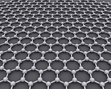
 Graphene is a material that is extracted from graphite and is made up of pure carbon, one of the most important elements in nature and which we find in daily objects like the lead of a pencil.

 Graphene (/ˈɡræfiːn/)^[1] is a carbon allotrope consisting of a single layer of atoms arranged in a honeycomb planar nanostructure.^[2][3] The name "graphene" is derived from "graphite" and the suffix -ene, indicating the presence of double bonds within the carbon structure. 

 

 

Now, we will calculate  its band structure and we need to do many calculations using different input files

graphene_scf.in

&CONTROL
  calculation = 'scf',
  prefix      = 'graphene',
  outdir      = '/tmp/',
  pseudo_dir  = './',
/

&SYSTEM
  ibrav     = 4,
  celldm(1) = 4.654,
  celldm(3) = 3.0,
  nat  = 2,
  ntyp = 1,
  ecutwfc = 40.0,
  ecutrho = 400.0,
  occupations = 'smearing',
  smearing = 'gaussian',
  degauss = 0.01,
/

&ELECTRONS
  conv_thr = 1.0d-8
/

ATOMIC_SPECIES
  C  12.0107 C.pbe-rrkjus.UPF

ATOMIC_POSITIONS alat
  C    0.000000    0.0000000   0.000000
  C    0.000000    0.5773503   0.000000

K_POINTS automatic
  9 9 1   0 0 0

You can download the pseudopotential from here C.pbe-rrkjus.UPF

Run the scf calculation 

pw.x -i graphene_scf.in > graphene_scf.out

 

graphene_nscf.in

&CONTROL
  calculation = 'nscf',
  prefix      = 'graphene',
  outdir      = '/tmp/',
  pseudo_dir  = './',
/

&SYSTEM
  ibrav     = 4,
  celldm(1) = 4.654,
  celldm(3) = 3.0,
  nat  = 2,
  ntyp = 1,
  ecutwfc = 40.0,
  ecutrho = 400.0,
  occupations='tetrahedra_opt'
/

&ELECTRONS
  conv_thr = 1.0d-8
/

ATOMIC_SPECIES
  C  12.0107 C.pbe-rrkjus.UPF

ATOMIC_POSITIONS alat
  C    0.000000    0.0000000   0.000000
  C    0.000000    0.5773503   0.000000

K_POINTS automatic
  12 12 1 0 0 0

 

Next increase the k-grid, and perform the non-self-consistent field calculation.

pw.x -i graphene_nscf.in > graphene_nscf.out

graphene_bands.in

&CONTROL
  calculation = 'bands',
  prefix      = 'graphene',
  outdir      = '/tmp/',
  pseudo_dir  = './',
/

&SYSTEM
  ibrav     = 4,
  celldm(1) = 4.654,
  celldm(3) = 3.0,
  nat  = 2,
  ntyp = 1,
  ecutwfc = 40.0,
  ecutrho = 400.0,
  nbnd=8
!  occupations = 'tetrahedra'
/

&ELECTRONS
  conv_thr = 1.0d-8
/

ATOMIC_SPECIES
  C  12.0107 C.pbe-rrkjus.UPF

ATOMIC_POSITIONS {alat}
  C    0.000000    0.0000000   0.000000
  C    0.000000    0.5773503   0.000000

K_POINTS {crystal_b}
4
  0.0000000000     0.0000000000     0.0000000000     20  ! Gamma
  0.3333333333     0.3333333333     0.0000000000     10  ! K
  0.0000000000     0.5000000000     0.0000000000     17  ! M
  0.0000000000     0.0000000000     0.0000000000     0   ! Gamma

 Run the bands calculation for given k-path:

pw.x -i graphene_bands.in > graphene_bands.out

 

graphene_bands_pp.in

&BANDS
  prefix  = 'graphene'
  outdir  = '/tmp/'
  filband = 'graphene_bands.dat'
  lsym = .true.,
/

 

Followed by the postprocessing to collect the bands:

bands.x -i graphene_bands_pp.in > graphene_bands_pp.out

 

 Make plot using the Matplotlib package and the script graphene-bands.py

To install the package we run the following command:

sudo apt-get install python3-matplotlib

 

 graphene-bands.py

import numpy as np
import matplotlib.pyplot as plt

data = np.loadtxt('./graphene_bands.dat.gnu')

k = np.unique(data[:, 0])
bands = np.reshape(data[:, 1], (-1, len(k)))

for band in range(len(bands)):
    plt.plot(k, bands[band, :], linewidth=1, alpha=0.5, color='k')
plt.xlim(min(k), max(k))

# Fermi energy
plt.axhline(0.921, linestyle=(0, (8, 10)), linewidth=0.75, color='k', alpha=0.5)
# High symmetry k-points (check bands_pp.out)
plt.axvline(0.6667, linewidth=0.75, color='k', alpha=0.5)
plt.axvline(1, linewidth=0.75, color='k', alpha=0.5)
# text labels
plt.xticks(ticks= [0, 0.6667, 1, 1.5774], labels=['$\Gamma$', 'K', 'M', '$\Gamma$'])
plt.ylabel("Energy (eV)")
plt.show()

 

To execute the script we run the following commands:

/Si-cutoff-pwtk$ python3 graphene-bands.py

We get the following picture: