 Recently
I have been using Quantum Espresso, which is an excellent piece of
software for running, electronic structure calculations. It is based on
density-functional theory, plane waves, and pseudopotentials.
Recently
I have been using Quantum Espresso, which is an excellent piece of
software for running, electronic structure calculations. It is based on
density-functional theory, plane waves, and pseudopotentials.
But it’s not very easy to use. Writing an input file, then analysing the output result becomes cumbersome.
So I started looking for alternative softwares that could do all this in an easy way. And I stumbled upon BURAI.
It’s a remarkable GUI for Quantum Espresso. You can build the input file using it’s intuitive and easy to use Graphical Interface. Then the results are also very neatly shown, like the Band Structure, Density of States, etc.
The best part is it comes with Quantum Espresso included, so it can
run all the Quantum Espresso calculations, and show you the results.
BURAI is available for Windows as well as MAC OS X.
PERSONAL NOTE: I also find BURAI helpful, as it is the only software
that I could, in my limited knowledge, use to run Quantum Espresso on
Windows. Before this I used to run the calculations on Linux.
In this post I will show you how to run some calculations and view the Results.
BURAI Home page: http://nisihara.wixsite.com/burai
Download the executable from: http://nisihara.wixsite.com/burai/resources
In my case I am using a Windows PC so I got the Windows version.
Once downloaded, the file would probably be around 250MB and compressed as a zip file. Unzip the file contents, to a location of your choice.
There is no need of installing with the package provided. You just go to the bin directory and launch the .exe:
BURAI1.2_Windows/bin/BURAI.exe
When you launch the application, it will look something like this:

You can click on the directory Examples, which contains different kinds of examples.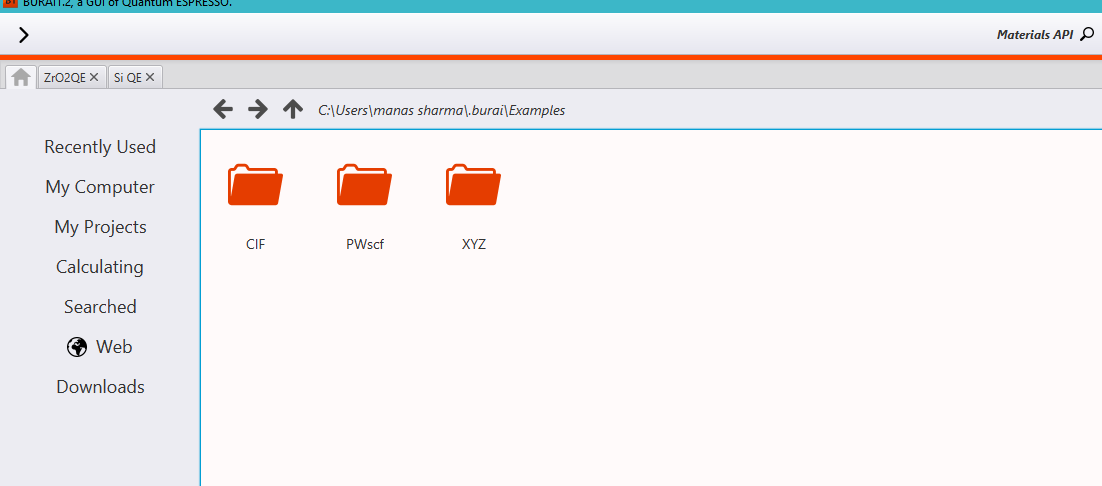
The directory called ‘CIF’ contains .cif files for some atoms/molecules.(CIF=Crystallographic Information File)
The directory called ‘PWscf’ contains Quantum Espresso example input files.
And the directory, ‘XYZ’ contains the .xyz files.
For the sake of this tutorial, let’s say you went ahead and clicked on ‘CIF’ and opened the file Fe.cif

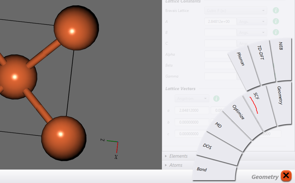
Once you open the file, it will look as shown above.
On the lower right corner you will see written, ‘Geometry’. What this
means is that you can adjust and specify various Geometry related
options in the options menu at the right of the window. You can specify
things like, lattice type, atomic positions, lattice parameters, etc.
For now, we would just let the things be the way they are.
Let’s now run an SCF calculation.
To do that click on the icon shown in the lower-right corner as shown in the picture.

A bunch of options should now pop-up as shown in the picture below. Choose SCF from them.
Once you click on SCF, you will see the options menu on the right would be replaced by new options. And now you can use this window to specify parameters for the SCF calculation. For now I will assume, that you know what each of those options mean. If you don’t know that, then you can refer to my other post on QE input file.
Now click on the button at the lower-left corner of the screen, as shown in the picture below:
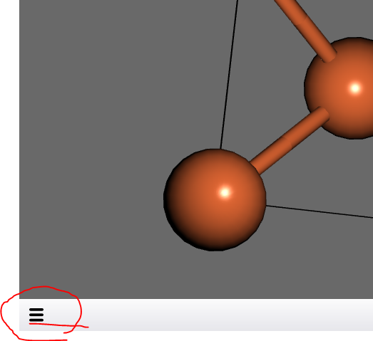
A small set of options will pop-up as shown:
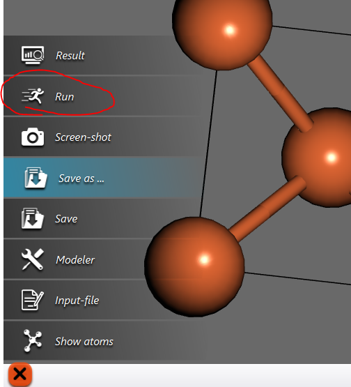
Now click on ‘Run’ to run an scf calculation.
When you click on ‘Run’, a small window will pop-up prompting you to save the project.

Leave the settings unchanged, and save the project.
Once you save the project, the job(scf calculation) will now run.
To view the result, click on the icon at the lower-left corner again, and this time choose ‘Result’ from the given options:
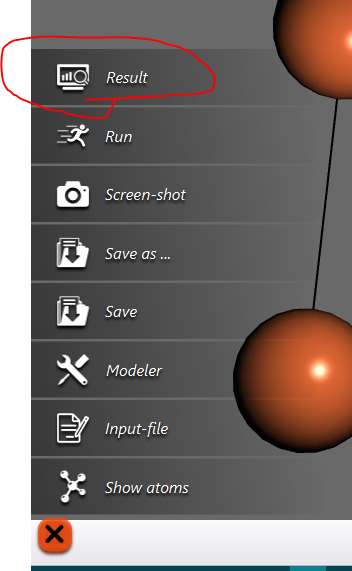
Once you click on result you will see some files as shown below:
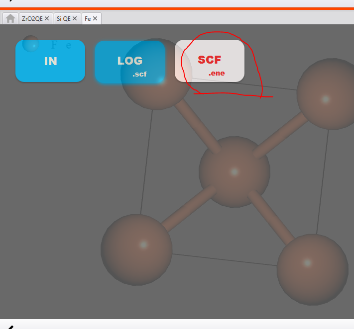
The result of the scf calculation is in a file called ‘SCF.ene’. It might take a few seconds for this file to appear. Just wait patiently.
Once you click on this file, you will see a graph of energy values obtained at each iteration as shown below:
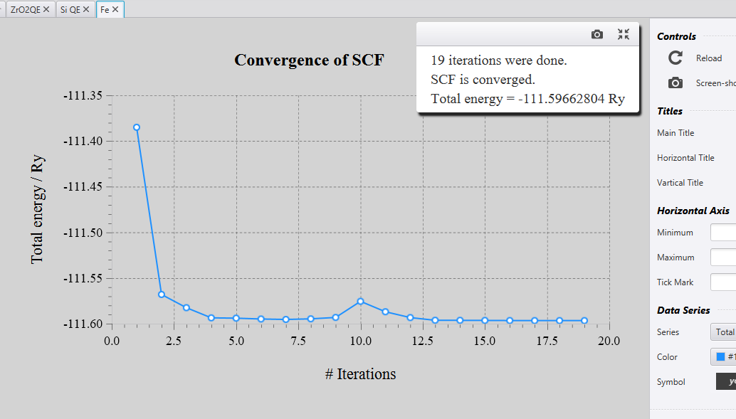
If the calculations are complete, it will show you ‘SCF is converged’ and you can note the energy.
If the calculations are not complete yet, it will show ‘SCF is not
converged’. In that case you can click on ‘Reload’ in the right of the
graph, to update the graph for the new iteration.
Well, that’s it!
That’s how you run a simple SCF calculation using BURAI.
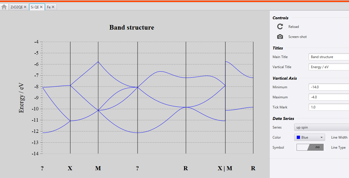
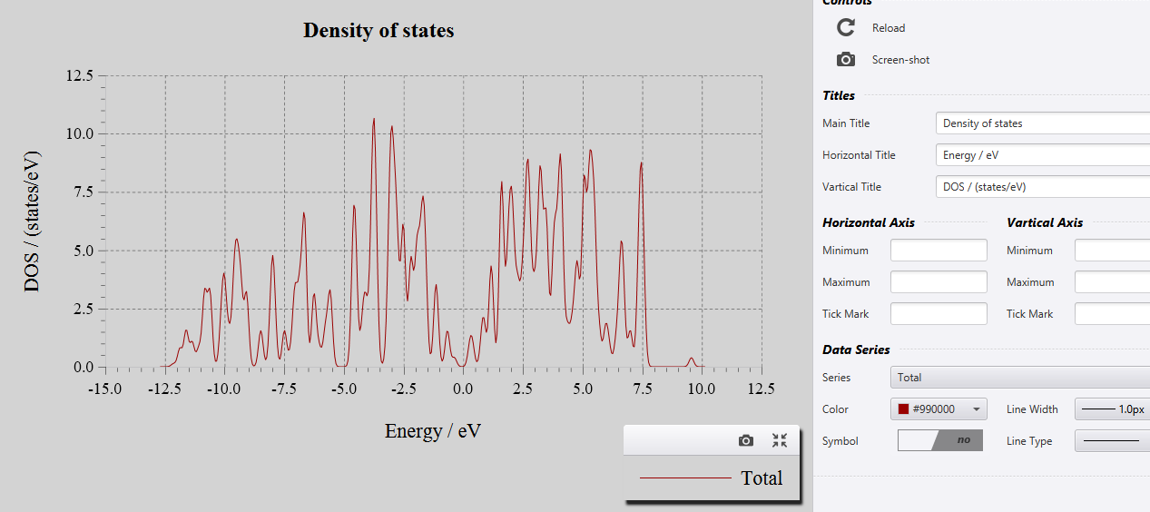
You can run more jobs like, Band Structure Calculation, Density of States calculations, etc in the same manner.
When you run ‘Band Structure’ and ‘DOS’ calculations, you will see the following files in the result section.
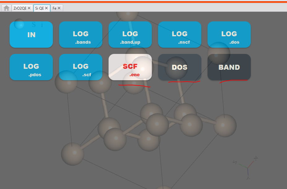
The results are in the file called ‘DOS’ and ‘BANDS’.
When you click on those you will see the output as shown below:
Hope you found this article useful!
If you have any questions/doubts leave them in the comments section down below.
https://www.bragitoff.com/2017/06/burai-1-2-gui-quantum-espresso-tutorial/


0 Comments